

Think quarterly forecasts can handle 2026 demand volatility? Think again.
Tariff swings, social-media spikes, shorter product lifecycles, and supplier churn made forecasting continuous, not a quarterly box-ticking exercise.
That matters because stockouts and dead stock now move faster than review cycles and directly hit revenue and margin.
Here’s the thesis: AI and machine-learning methods, demand sensing, probabilistic forecasting, and ML ensembles let you update forecasts daily, measure uncertainty, and cut inventory cost without blowing service levels.
Read on for practical steps to start in days, not quarters.
Immediate Solutions for Handling 2026 Demand Volatility with Modern Inventory Forecasting

Forecasting changed between 2023 and 2026. What used to be a quarterly task is now continuous. Tariff swings, monthly supply disruptions, shorter product lifecycles, social media demand spikes. Traditional quarterly cycles can’t keep up. Locking a forecast at quarter start and executing against it? That leaves you exposed. Shortages, excess stock, missed margin. The volatility isn’t slowing down. It’s the baseline now.
The shift is toward AI-driven, adaptive systems. Machine learning pattern recognition, demand sensing from real-time signals, scenario-based planning. Top performers update forecasts 3.2 times more often than average ones. They maintain forecast accuracy 23 percent higher. They run four to six demand scenarios at once (baseline, optimistic, conservative) with predefined triggers to switch plans. They adopt AI forecasting tools at nearly double the rate: 48 percent versus 23 percent. They treat forecasting as a decision platform, not just a planning document.
The core methods that work for 2026 volatility:
AI-powered forecasting: Large-scale pattern recognition across SKUs, channels, external signals.
Machine learning ensembles: Combining multiple statistical and ML models for accuracy under varying conditions.
Probabilistic forecasting: Modeling demand as a distribution, not a single number. Captures uncertainty and sets safety stock accordingly.
Demand sensing: Real-time adjustments using POS data, digital behavior, weather, promotions. Shortens planning cycles.
Rapid-cycle updates: Weekly or daily forecast refreshes for key SKUs instead of monthly or quarterly reviews.
The measurable difference is clear. Leading teams don’t wait for perfect data or precise models. An 80 percent accurate forecast updated weekly beats a 90 percent accurate forecast updated monthly. AI handles large-scale pattern detection (seasonality, promotions, cross-SKU relationships) while human planners apply business context and adjust outliers the system flags. Speed and responsiveness matter as much as precision now.
Modern Inventory Forecasting Approaches That Replace Traditional Methods

Traditional methods relied on historical averages, moving averages, ARIMA models. They assume stable patterns and limited external shocks. That works when demand is predictable and supply is stable. In 2026, neither holds true. History-based forecasting treats the past as the best predictor of the future. But when tariffs shift monthly, product lifecycles compress, customer behavior responds to social media in real time? The past becomes a poor guide.
Modern forecasting is adaptive and data-driven. It uses machine learning ensembles, deep learning networks, Bayesian models, generative simulations. Detects patterns that change faster than quarterly cycles. AI-powered forecasting has demonstrated measurable gains: roughly 30 percent reduction in inventory levels, 20 percent reduction in logistics costs, 15 percent reduction in procurement spend when embedded into operations. These aren’t theoretical improvements. They reflect implementations where continuous recalculation, external signal ingestion, probabilistic modeling replaced static spreadsheets.
| Method | Best Use Case | Volatility Suitability |
|---|---|---|
| ML Ensembles | High-velocity SKUs with multiple causal drivers | High, adapts to pattern shifts |
| Probabilistic Models | Setting safety stock and service levels | High, captures uncertainty as distributions |
| Deep Learning Networks (LSTM, Transformer) | Complex, cross-SKU patterns and long sequences | Very High, detects non-linear relationships |
| Bayesian Models | Incorporating prior knowledge and small datasets | Medium-High, updates beliefs with new data |
| Intermittent-Demand Models (Croston’s) | Sporadic sales and long-tail SKUs | Medium, smooths irregular demand intervals |
Under high volatility, deep learning networks and ML ensembles outperform traditional statistical models. They continuously retrain as new data arrives. They can handle large numbers of exogenous variables (promotions, competitor pricing, weather, supplier delays) without manual feature selection. Bayesian models let planners incorporate domain knowledge and update forecasts as evidence accumulates. Valuable when launching new products or entering new markets with limited history. Intermittent-demand models address the long tail of SKUs with sporadic sales, where standard time-series methods fail.
Real-Time Demand Sensing and Data Signals for 2026 Inventory Forecasting

Real-time demand sensing adjusts forecasts based on signals that arrive hourly or daily. It doesn’t wait for end-of-month sales reports. Treats forecasting as a continuous process, not a batch task. Demand sensing shortens reaction time between a market shift and an operational response. Critical when lead times are weeks or months and inventory decisions lock in capital.
The most valuable real-time signals for 2026 forecasting:
Point-of-sale data: Actual sell-through at retail or online, updated daily or intraday. Detects demand acceleration or deceleration.
Digital browsing and search behavior: Click-through rates, product-page views, cart additions, search volume as leading indicators of purchase intent.
Weather forecasts and events: Temperature shifts, storms, seasonal changes that affect categories like apparel, food, outdoor goods.
Social media shifts: Viral trends, influencer mentions, sentiment changes driving sudden spikes in specific SKUs.
Promotion telemetry: Real-time performance of discounts, bundles, campaigns. Adjusts forecasts before inventory commits.
Supplier lead-time changes: Alerts from suppliers or carriers about delays, capacity constraints, tariff impacts that alter replenishment timing.
Leading organizations use daily or weekly adjustments for key SKUs. An automotive parts distributor supporting 50 service centers moved from quarterly reviews to daily transfer decisions. Reduced stockouts and reallocated inventory based on live demand. A food and beverage manufacturer managing over 800 SKUs instituted a weekly cadence. Adjusted for shelf-life constraints and promotional performance. In both cases, real-time signals replaced lagging indicators. Cut planning cycles from weeks to days. The faster the cycle, the less buffer inventory is needed to cover uncertainty.
Probabilistic and Scenario-Based Inventory Forecasting Models for Volatile Markets

Point forecasts fail in volatility. They provide a single number with no information about uncertainty. A forecast of 1,000 units could mean high confidence in a narrow range or a wide distribution spanning 500 to 1,500 units. Without knowing the distribution, planners can’t set appropriate safety stock, service levels, purchasing decisions. Probabilistic forecasting models the demand as a range with associated probabilities. Operators can quantify risk and make trade-offs between cost and service.
Monte Carlo simulation, Bayesian inference, ensemble modeling generate probabilistic ranges rather than point estimates. These methods run thousands of scenarios to produce a forecast distribution. Scenario-based forecasting extends this by creating distinct demand paths (baseline, optimistic, conservative) and defining operational triggers to switch plans when market signals cross predefined thresholds. Top performers run four to six scenarios in parallel. Use scenario engines to reveal impacts on inventory, service levels, cost before decisions are finalized. For example, a baseline scenario might assume moderate growth. An optimistic scenario models a successful product launch or viral social trend. When early sales data confirm one scenario over another, inventory plans adjust within the same week.
Practical applications of probabilistic and scenario-based forecasting:
Service level tuning: Setting different service targets for high-margin versus commodity SKUs based on the cost of a stockout versus the cost of excess inventory.
Safety stock setting: Calculating buffer inventory as a function of demand variability and lead-time uncertainty, not a fixed percentage of average demand.
Buffer strategy evaluation: Comparing the cost of holding intentional excess inventory as “insurance” against the cost of lost sales and expedited freight when stockouts occur.
Risk-adjusted purchasing: Committing purchase orders only after probabilistic models confirm demand strength. Reduces exposure to dead stock from optimistic forecasts.
Scenario planning isn’t academic. It’s operational. When tariffs shift or a competitor exits a category, scenario models let operators reforecast and replan in days, not months.
Safety Stock and Buffer Inventory Optimization for 2026 Volatility

Safety stock in stable markets was a simple formula: average demand times a fixed multiplier. In 2026, that approach ties up cash and still generates stockouts. The multiplier doesn’t adjust to real-time volatility. Q2 2025 saw a rise in intentional buffer stock strategies as “insurance” against supply disruptions. But without risk modeling, those buffers often became dead stock. Forecasting error directly ties to carrying cost and capital usage. Top performers balance intentional excess with accurate demand sensing. Recalculating safety stock weekly or more frequently for high-volatility SKUs.
Dynamic safety stock calculation uses the forecast distribution, not a point estimate. Determines how much buffer is needed to hit a target service level. If demand variability increases or supplier lead times extend, safety stock rises automatically. If demand stabilizes or a supplier improves reliability, the buffer shrinks. Frees working capital. This requires real-time visibility into both demand signals and supply signals (late shipments, port delays, tariff changes) so the safety stock formula reflects current conditions.
| Volatility Condition | Recommended Method | Inventory Impact |
|---|---|---|
| High demand variance, stable lead time | Increase safety stock based on demand distribution | Moderate increase |
| Stable demand, long or variable lead time | Increase safety stock based on lead-time distribution | Moderate to high increase |
| High demand variance and variable lead time | Combine demand and lead-time uncertainty; use probabilistic models | High increase; requires scenario planning |
Risk-modeled buffers improve service levels without over-investing in inventory. They shift the question from “How much should we hold?” to “What service level can we afford, and what does that cost?” When carrying cost, stockout cost, forecast uncertainty are quantified, operators make informed trade-offs. For high-margin SKUs with short lifecycles, higher safety stock may be justified. For commodity SKUs with low margins, lower service levels and minimal buffers make more sense. The model makes the trade-off visible before the purchase order is signed.
Multi-Echelon Inventory Optimization and SKU-Level Forecasting in 2026

Multi-echelon forecasting manages inventory across warehouse, regional distribution centers, retail or e-commerce nodes as a network. Not independent locations. Aggregate forecasting at the network level hides item-level risks. A total forecast might look healthy while individual SKUs are overstocked in one region and out of stock in another. SKU-level visibility is essential because it reveals where demand is actually happening and where inventory is sitting idle. An automotive parts distributor supporting 50 service centers moved to daily transfer decisions at the SKU level. Reallocating inventory based on live demand rather than static allocation rules. A food and beverage manufacturer managing over 800 SKUs instituted a weekly cadence. Adjusted for shelf-life constraints, ensuring fresh product reached stores without waste.
Multi-echelon optimization delivers measurable benefits:
Lower network-wide inventory: Safety stock is pooled at higher echelons. Reduces total system stock while maintaining service levels.
Reduced transfer delays: Real-time SKU-level forecasts trigger proactive transfers before stockouts occur at downstream nodes.
Fewer stockouts: Demand is sensed closer to the customer. Inventory is repositioned faster.
Optimized cash flow: Capital isn’t locked in slow-moving SKUs at distant warehouses while fast movers run out at high-velocity locations.
SKU-level methods differentiate forecast horizon, lead-time variability, velocity tiers. High-velocity SKUs receive daily or weekly updates using machine learning and real-time demand sensing. Medium-velocity SKUs use weekly or biweekly statistical models. Long-tail SKUs with intermittent demand use Croston’s method or simple moving averages, with longer review cycles to avoid overreaction to noise. Lead-time variability is modeled at the SKU-supplier pair level. Safety stock reflects the actual reliability of each supply source. This granularity prevents the one-size-fits-all approach that either overstocks slow movers or understocks fast movers.
Forecast Accuracy Metrics and Error Reduction for 2026 Inventory Planning
Forecast accuracy metrics quantify how well predictions match actual demand. They identify where models need improvement. Top performers hit accuracy rates 20 to 25 percent higher than average performers. Update forecasts 3.2 times more frequently. Data quality issues plague average performers. Top performers focus on external signal ingestion and outlier management. Accuracy alone isn’t the goal. The goal is operational performance: fewer stockouts, lower carrying costs, faster responses to market shifts.
Key metrics for 2026 inventory forecasting:
MAPE (Mean Absolute Percentage Error): Average percentage difference between forecast and actual demand. Easy to interpret but can be distorted by low-volume SKUs.
WAPE (Weighted Absolute Percentage Error): Similar to MAPE but weighted by sales volume. Gives more weight to high-revenue SKUs.
MASE (Mean Absolute Scaled Error): Compares forecast error to a naive baseline (such as last year’s demand). Values below 1 indicate the model outperforms the naive method.
Forecast bias: Measures whether the model consistently over-forecasts or under-forecasts. Bias indicates systematic errors that need correction.
Service-level impact metrics: Stockout rate, fill rate, lost-sales dollars tied directly to forecast error. Shows the business cost of inaccuracy.
Anomaly detection and outlier handling prevent rare events from skewing the entire forecast. Outliers (such as a one-time bulk order or a promotional spike) are flagged. Either excluded from historical training data or modeled separately. Machine learning models can learn which events are true demand signals and which are noise. But only if the training data is clean. Average performers struggle with dirty data: duplicate records, missing POS feeds, promotion flags not captured in the system. Top performers invest in data pipelines, governance, lineage so that every forecast input is traceable and validated.
Update frequency directly affects accuracy. A forecast refreshed weekly with the latest POS data, promotion performance, supplier alerts will outperform a monthly forecast built on stale data. Even if the monthly forecast uses a more sophisticated model. Leading organizations update high-velocity SKUs daily or weekly, medium-velocity SKUs weekly or biweekly, long-tail SKUs monthly. The update cadence is set by the speed of demand change, not by the calendar.
Data Quality, Feature Engineering, and ERP Integration for 2026 Forecasting Models

Poor historical data is the top challenge cited by average performers. Missing records, inconsistent SKU identifiers, promotion flags not tied to sales transactions, supplier lead times recorded manually in spreadsheets. All of this degrades model accuracy. Top performers invest in external-signal ingestion: promotions, competitor actions, supplier status updates, tariff announcements, weather forecasts. They treat data quality as a prerequisite for forecasting, not an afterthought. Clean, timely, complete data is the foundation. Without it, even the most advanced machine learning models produce unreliable outputs.
Most ERPs are described as “broad but shallow” for forecasting. They track on-hand inventory, process transactions, generate basic demand reports. But they lack advanced scenario modeling, probabilistic forecasting, real-time demand sensing. Common ERP pairings include Business Central, Dynamics 365 Finance and Supply Chain, Dynamics GP, SAP Business One. Leading organizations integrate specialized forecasting platforms with their ERP. Preserves transactional integrity while gaining advanced analytics. The ERP remains the system of record for inventory levels, purchase orders, sales transactions. The forecasting platform ingests that data, adds external signals, runs machine learning models, pushes recommended orders back to the ERP for execution.
Engineering the Right Inputs for Modern Forecasting Models
Feature engineering transforms raw data into inputs that machine learning models can use. Causal variables (price changes, promotional discounts, competitor activity, new product launches) are encoded as features. Weather signals are mapped to relevant SKUs: temperature for beverages, precipitation for outdoor gear, seasonal transitions for apparel. Promotions are tagged with start date, discount depth, channel, expected lift. Supplier risk data (on-time delivery rate, lead-time variability, port congestion) are incorporated to adjust safety stock and reorder points.
Exogenous variables improve forecast accuracy by giving models information that isn’t visible in historical sales alone. For example, a spike in demand during a past promotion isn’t just “high sales in week 23” but “high sales during a 20 percent off promotion running on social media.” The model learns the relationship between discount depth and demand lift. Enables it to forecast the impact of future promotions. Lead-time fluctuations are modeled as distributions, not fixed numbers. Safety stock adjusts when a supplier’s lead time becomes more variable. External economic indicators (GDP growth, unemployment, consumer sentiment) can be included for SKUs sensitive to macroeconomic conditions.
ERPs integrate with modern forecasting platforms through automated data pipelines. Real-time or near-real-time feeds pull sales transactions, inventory levels, purchase orders, receipts. The forecasting platform processes those inputs, generates updated forecasts, surfaces recommended actions (purchase orders, transfer orders, safety stock adjustments) through dashboards and automated alerts. When a forecast detects an anticipated stockout or excess inventory building, the system flags it before capital is committed. The integration is bidirectional: the ERP provides data, and the forecasting platform provides decision intelligence that informs purchasing, allocation, replenishment.
Implementation Roadmap: Moving to 2026-Ready Inventory Forecasting
Organizational readiness and training are prerequisites for successful implementation. Forecasting isn’t just a technology upgrade. It requires cross-functional alignment between supply chain, sales, finance, executive leadership. Training planners in statistical methods and commercial judgment ensures AI-generated forecasts are understood, trusted, adjusted when business context demands it. Top performers have 67 percent of leading planners reporting directly to executive leadership, versus 41 percent for average performers. This ensures forecasting insights inform strategic decisions on capital allocation, growth, risk.
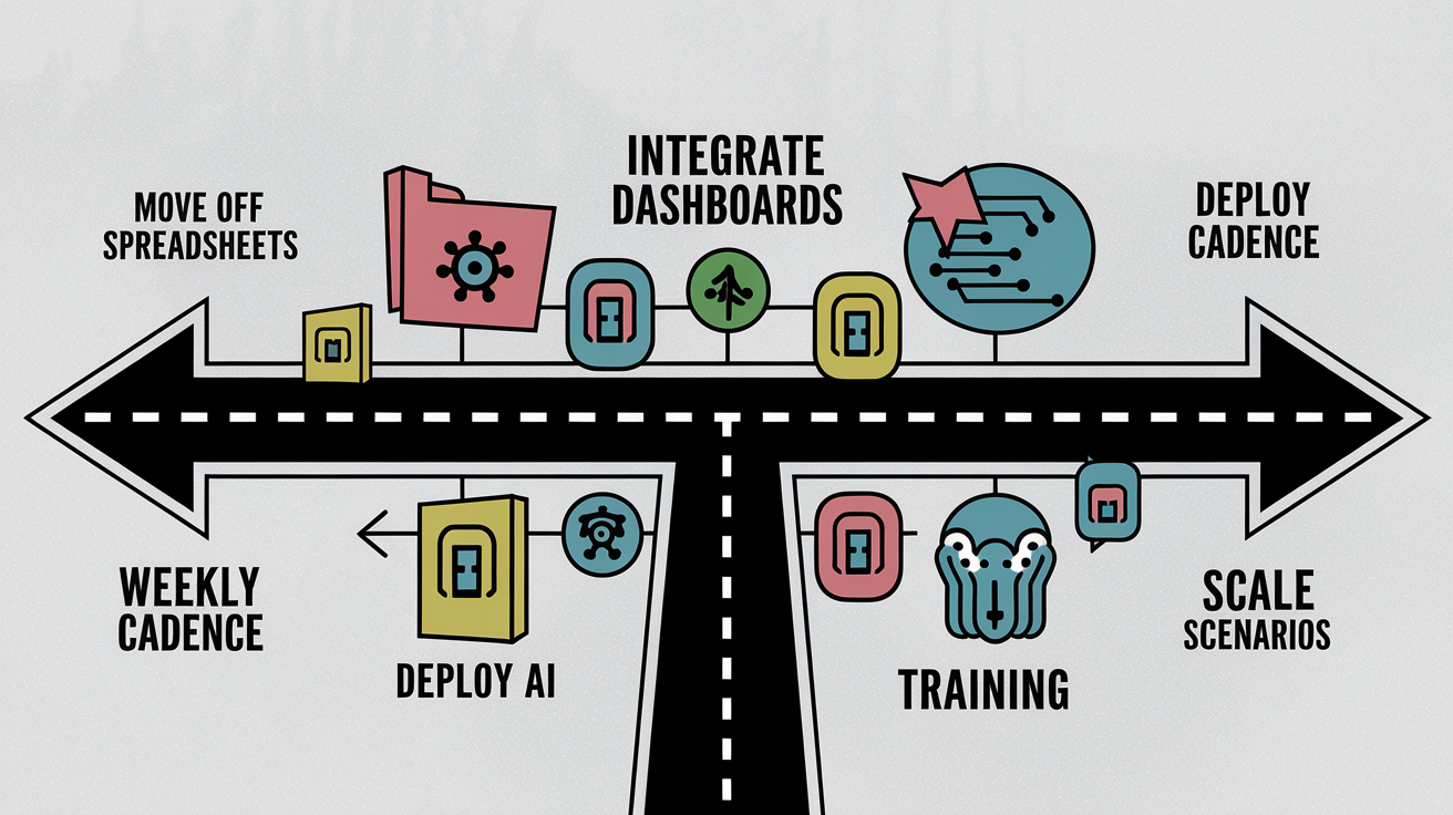
The implementation sequence:
Move off spreadsheets to an integrated demand-planning platform: Replace manual Excel-based forecasting with a dedicated platform that automates data ingestion, model execution, scenario planning.
Automate data ingestion and build real-time dashboards: Connect POS, ERP, supplier feeds, external signals into a unified data pipeline. Create dashboards that surface forecast accuracy, inventory levels, exception alerts.
Deploy AI and machine learning for baseline forecasts and anomaly detection: Implement ML models that continuously retrain on new data and flag outliers or unexpected demand shifts for human review.
Institutionalize weekly cross-functional cadence and scenario planning: Hold weekly planning meetings with sales, operations, finance to review forecasts, adjust scenarios, align on decisions. Maintain four to six active scenarios with predefined triggers.
Train planners in statistical methods plus commercial judgment: Teach planners how to interpret probabilistic forecasts, understand model outputs, apply business context to adjust AI recommendations.
Scale scenario planning and continuous improvement practices: Expand scenario modeling to cover longer horizons and more SKUs. Establish monthly or quarterly reviews of model performance, forecast accuracy, process effectiveness.
Continuous improvement practices include model retraining frequency, dashboard reviews, feedback loops. High-velocity SKUs are retrained daily or weekly as new data arrives. Medium-velocity SKUs are retrained weekly or biweekly. Long-tail SKUs are retrained monthly or quarterly. Dashboard reviews happen weekly in top-performing organizations. Exception alerts trigger immediate action when forecasts deviate from actuals or when inventory risks exceed thresholds. Feedback loops capture planner adjustments (such as overriding a forecast based on a known promotional event) and feed those insights back into the model to improve future accuracy.
Case Studies and Industry Use Cases Demonstrating Forecasting Success in Volatile Markets
Quantified results from real-world implementations demonstrate the operational impact of advanced forecasting. A global luxury fashion retailer reduced lost sales by 11 million dollars in North America and 21 million dollars in EMEA by adopting AI-driven forecasting and real-time demand sensing. A multi-brand jewelry retailer got 22 million dollars in inventory savings across banners by moving from spreadsheet-based planning to a unified platform with SKU-level forecasts and scenario modeling. In some industries, AI-powered forecasting has reduced lost sales and product unavailability by 65 percent. Turning stockouts from a chronic problem into a rare exception.
Industry-specific examples:
Food and beverage manufacturer: Managing over 800 SKUs with a weekly forecasting cadence. Adjusts for shelf-life constraints, promotional performance, seasonal demand shifts.
Automotive parts distributor: Supporting 50 service centers with daily transfer decisions at the SKU level. Reallocating inventory based on live demand rather than static rules.
Luxury fashion retailer: Reducing lost sales by tens of millions of dollars through AI-driven demand sensing and real-time adjustments to replenishment plans.
Multi-brand jewelry retailer: Saving 22 million dollars in inventory by consolidating forecasting across banners. Using scenario planning to align purchasing with probabilistic demand.
These cases show that advanced forecasting isn’t theoretical. It delivers measurable improvements in service levels, inventory efficiency, cash flow when technology, process, skills are aligned. The organizations that move first (away from spreadsheets, toward real-time data, into scenario-based planning) gain a measurable advantage in 2026’s volatile markets.
Final Words
In the action, we showed why 2026 demand volatility breaks quarterly forecasts and what replaces them: AI/ML ensembles, demand sensing, probabilistic scenarios, rapid‑cycle updates, and SKU‑level, multi‑echelon rules. Top performers update forecasts 3.2× more often and run 4–6 scenarios.
Next steps: move to daily/weekly updates, pilot AI forecasting on your top 20 SKUs, set scenario triggers, and recalc safety stock dynamically. inventory forecasting methods for 2026 demand volatility are practical and measurable — you can start small and see faster wins.
FAQ
Q: What methods do you use to forecast inventory demand?
A: The methods I use to forecast inventory demand are demand sensing (real-time POS and digital signals), ML ensemble models, probabilistic (Monte Carlo) forecasts, scenario-based planning, and manual outlier review.
Q: What are the 4 forecasting methods?
A: The four forecasting methods are time-series statistical models (moving averages, ARIMA), causal regression models, machine-learning/AI ensembles, and probabilistic or scenario-based approaches that show forecast ranges.
Q: What are the methods of forecasting volatility?
A: The methods of forecasting volatility are probabilistic modeling and Monte Carlo simulation, volatility-aware stats (eg, GARCH), ML ensembles with uncertainty estimates, demand sensing, and scenario stress-testing.
Q: What are the 4 types of demand patterns?
A: The four types of demand patterns are stable (horizontal), trend (consistent up/down), seasonal (regular cycles), and intermittent or sporadic demand with many zero periods.